43 chart data labels excel
How to Create Charts in Excel (In Easy Steps) 1. Select the chart. 2. Click the + button on the right side of the chart, click the arrow next to Legend and click Right. Result: Data Labels. You can use data labels to focus your readers' attention on a single data series or data point. 1. Select the chart. 2. Click a green bar to select the Jun data series. 3. How to create Custom Data Labels in Excel Charts Add data labels Create a simple line chart while selecting the first two columns only. Now Add Regular Data Labels. Two ways to do it. Click on the Plus sign next to the chart and choose the Data Labels option. We do NOT want the data to be shown. To customize it, click on the arrow next to Data Labels and choose More Options …
How to add data labels from different column in an Excel ... Right click the data series in the chart, and select Add Data Labels > Add Data Labels from the context menu to add data labels. 2. Click any data label to select all data labels, and then click the specified data label to select it only in the chart. 3.
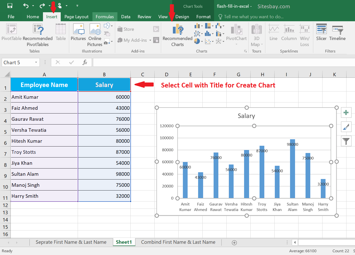
Chart data labels excel
How to hide zero data labels in chart in Excel? - ExtendOffice If you want to hide zero data labels in chart, please do as follow: 1. Right click at one of the data labels, and select Format Data Labels from the context menu. See screenshot: 2. In the Format Data Labels dialog, Click Number in left pane, then select Custom from the Category list box, and type #"" into the Format Code text box, and click Add button to add it to Type list box. Currency format on excel chart data label lost I have a workbook created in Excel 2013 with some charts which have data labels showing currency values. The workbook was created on my local machine, and when I refresh it on there it behaves as expected, and when I save it on Sharepoint I can see the £ symbol on the chart when I view it using excel services. Add or remove data labels in a chart Click the data series or chart. To label one data point, after clicking the series, click that data point. In the upper right corner, next to the chart, click Add Chart Element > Data Labels. To change the location, click the arrow, and choose an option. If you want to show your data label inside a text bubble shape, click Data Callout.
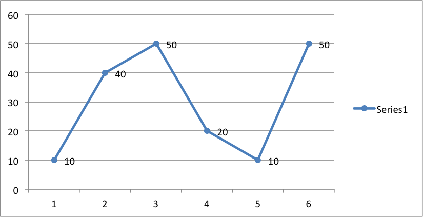
Chart data labels excel. How to Use Cell Values for Excel Chart Labels Select the chart, choose the "Chart Elements" option, click the "Data Labels" arrow, and then "More Options." Uncheck the "Value" box and check the "Value From Cells" box. Select cells C2:C6 to use for the data label range and then click the "OK" button. The values from these cells are now used for the chart data labels. How to Change Excel Chart Data Labels to Custom Values? First add data labels to the chart (Layout Ribbon > Data Labels) Define the new data label values in a bunch of cells, like this: Now, click on any data label. This will select "all" data labels. Now click once again. At this point excel will select only one data label. Add / Move Data Labels in Charts - Excel & Google Sheets ... Check Data Labels . Change Position of Data Labels. Click on the arrow next to Data Labels to change the position of where the labels are in relation to the bar chart. Final Graph with Data Labels. After moving the data labels to the Center in this example, the graph is able to give more information about each of the X Axis Series. How to Add Data Labels to an Excel 2010 Chart - dummies Excel provides several options for the placement and formatting of data labels. Use the following steps to add data labels to series in a chart: Click anywhere on the chart that you want to modify. On the Chart Tools Layout tab, click the Data Labels button in the Labels group. A menu of data label placement options appears: None: The default ...
How To Use Dynamic Data Labels To Create Interactive Excel ... If you are an Excel user then this blog is highly useful to you, here know how to create Dynamic Data Labels, which can be highlighted when they are needed the most.. In MS Excel worksheet Chart is a perfect tool to present data in an enhanced and more understandable way but most of the time it is seen that it stuck because of the overloading of the excess of data representation. Add data labels to your Excel bubble charts - TechRepublic If you want to add labels to the bubbles in an Excel bubble chart, you have to do it after you create the chart. Mary Ann Richardson explains what you need to do to add a data label to each bubble. Excel charts: how to move data labels to legend ... @Matt_Fischer-Daly . You can't do that, but you can show a data table below the chart instead of data labels: Click anywhere on the chart. On the Design tab of the ribbon (under Chart Tools), in the Chart Layouts group, click Add Chart Element > Data Table > With Legend Keys (or No Legend Keys if you prefer) How to add or move data labels in Excel chart? In Excel 2013 or 2016. 1. Click the chart to show the Chart Elements button . 2. Then click the Chart Elements, and check Data Labels, then you can click the arrow to choose an option about the data labels in the sub menu. See screenshot: In Excel 2010 or 2007. 1. click on the chart to show the Layout tab in the Chart Tools group. See ...
Change the format of data labels in a chart To get there, after adding your data labels, select the data label to format, and then click Chart Elements > Data Labels > More Options. To go to the appropriate area, click one of the four icons ( Fill & Line, Effects, Size & Properties ( Layout & Properties in Outlook or Word), or Label Options) shown here. Custom Data Labels with Colors and Symbols in Excel Charts ... The basic idea behind custom label is to connect each data label to certain cell in the Excel worksheet and so whatever goes in that cell will appear on the chart as data label. So once a data label is connected to a cell, we apply custom number formatting on the cell and the results will show up on chart also. Following steps help you ... Excel Charts - Aesthetic Data Labels - Tutorialspoint Data labels stay in place, even when you switch to a different type of chart. You can also connect the data labels to their data points with leader lines on all charts. Here, we will use a Bubble chart to see the formatting of data labels. Data Label Positions. To place the data labels in the chart, follow the steps given below. How to add total labels to stacked column chart in Excel? Add total labels to stacked column chart in Excel Supposing you have the following table data. 1. Firstly, you can create a stacked column chart by selecting the data that you want to create a chart, and clicking Insert > Column, under 2-D Column to choose the stacked column. See screenshots: And now a stacked column chart has been built. 2.
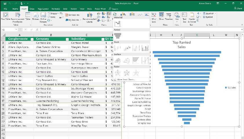
How to Create Chart in Excel - Excel Tutorial
Chart.ApplyDataLabels method (Excel) | Microsoft Docs For the Chart and Series objects, True if the series has leader lines. Pass a Boolean value to enable or disable the series name for the data label. Pass a Boolean value to enable or disable the category name for the data label. Pass a Boolean value to enable or disable the value for the data label.
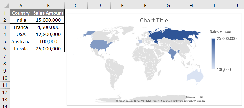
Map Chart in Excel | Steps to Create Map Chart in Excel with Examples
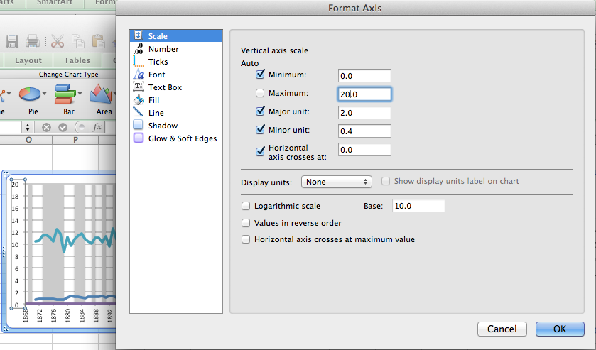
How to format axis labels as thousands/millions in Excel? Right click at the axis you want to format its labels as thousands/millions, select Format Axisin the context menu. 2. In the Format Axisdialog/pane, click Number tab, then in theCategorylist box, select Custom, and type[>999999] #,,"M";#,"K"into Format Codetext box, and click Addbutton to add it toTypelist. See screenshot: 3.

Enable or Disable Excel Data Labels at the click of a button - How To - PakAccountants.com
Edit titles or data labels in a chart - support.microsoft.com On a chart, click one time or two times on the data label that you want to link to a corresponding worksheet cell. The first click selects the data labels for the whole data series, and the second click selects the individual data label. Right-click the data label, and then click Format Data Label or Format Data Labels.
Data Callout Excel 2019 Mac - greenwaymedicine
vb.net excel chart data label positioning Hi, I have exported an Excel chart from my winform app and added some data labels to each point. You can manually drag these data labels anywhere you want on the Excel chart but I would like to programmatically set them all to be displayed at the bottom of the chart (I have hidden the x axis labels so ideally where these would normally be displayed).

Excel Chart Not Showing All Data Labels - Chart Walls
Add or remove data labels in a chart Click the data series or chart. To label one data point, after clicking the series, click that data point. In the upper right corner, next to the chart, click Add Chart Element > Data Labels. To change the location, click the arrow, and choose an option. If you want to show your data label inside a text bubble shape, click Data Callout.

How to Change Excel Chart Data Labels to Custom Values? | Chandoo.org - Learn Microsoft Excel Online
Currency format on excel chart data label lost I have a workbook created in Excel 2013 with some charts which have data labels showing currency values. The workbook was created on my local machine, and when I refresh it on there it behaves as expected, and when I save it on Sharepoint I can see the £ symbol on the chart when I view it using excel services.
Adding Colored Regions to Excel Charts - Duke Libraries Center for Data and Visualization Sciences
How to hide zero data labels in chart in Excel? - ExtendOffice If you want to hide zero data labels in chart, please do as follow: 1. Right click at one of the data labels, and select Format Data Labels from the context menu. See screenshot: 2. In the Format Data Labels dialog, Click Number in left pane, then select Custom from the Category list box, and type #"" into the Format Code text box, and click Add button to add it to Type list box.
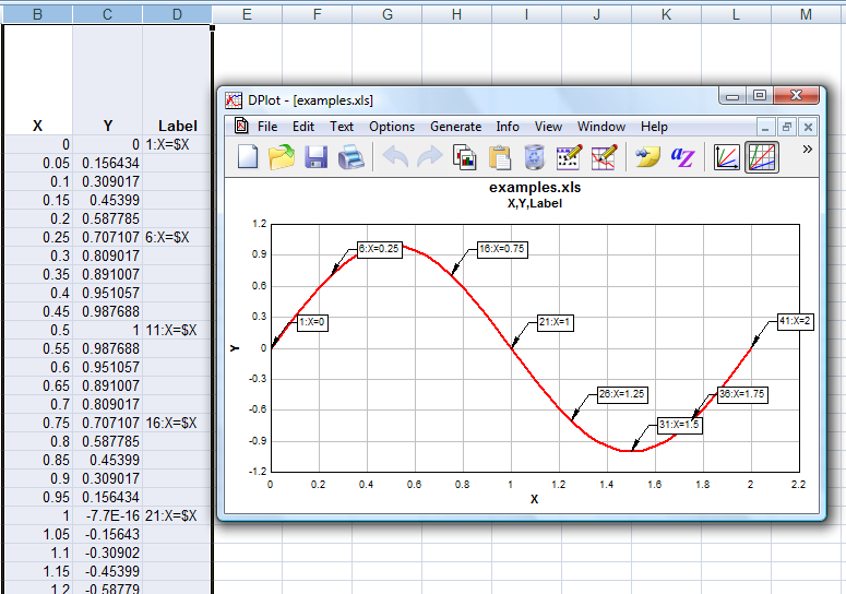
DPlot Windows software for Excel users to create presentation quality graphs
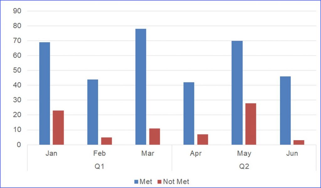
How to Create a Chart with the Axis having Two Categories - ExcelNotes
![Custom Data Labels with Colors and Symbols in Excel Charts - [How To] - PakAccountants.com](http://pakaccountants.com/wp-content/uploads/2014/09/data-label-chart-4.gif)
Custom Data Labels with Colors and Symbols in Excel Charts - [How To] - PakAccountants.com
Working with Charts — XlsxWriter Documentation

Data labels on Excel charts « projectwoman.com

Sunburst Charts and Treemaps (Excel 2016+) | Microsoft Excel - Dashboards
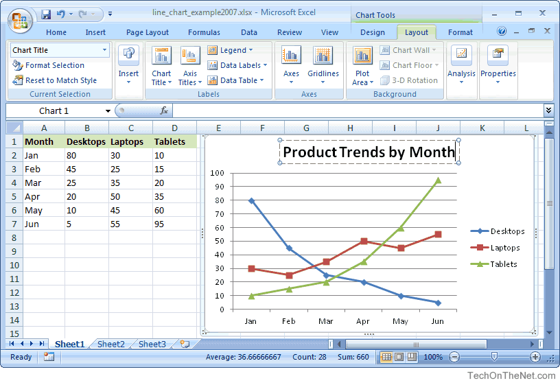
MS Excel 2007: How to Create a Line Chart
Post a Comment for "43 chart data labels excel"