41 excel chart multiple data labels

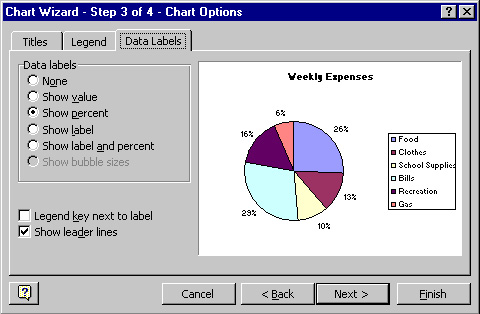
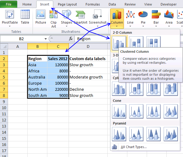
Chart.ApplyDataLabels method (Excel) | Microsoft Docs Syntax expression. ApplyDataLabels ( Type, LegendKey, AutoText, HasLeaderLines, ShowSeriesName, ShowCategoryName, ShowValue, ShowPercentage, ShowBubbleSize, Separator) expression A variable that represents a Chart object. Parameters Example This example applies category labels to series one on Chart1. VB Copy Charts ("Chart1").SeriesCollection (1). How to Create Charts in Excel: Types & Step by Step Examples Open Excel. Enter the data from the sample data table above. Your workbook should now look as follows. To get the desired chart you have to follow the following steps. Select the data you want to represent in graph. Click on INSERT tab from the ribbon. Click on the Column chart drop down button.

› data-series-data-points-dataUnderstanding Excel Chart Data Series, Data Points, and Data ... Sep 19, 2020 · When multiple data series are plotted in one chart, each data series is identified by a unique color or shading pattern. Not all graphs include groups of related data or data series. In column or bar charts, if multiple columns or bars are the same color or have the same picture (in the case of a pictograph ), they comprise a single data series.

Excel chart multiple data labels

How to Add Labels to Scatterplot Points in Excel - Statology Step 3: Add Labels to Points Next, click anywhere on the chart until a green plus (+) sign appears in the top right corner. Then click Data Labels, then click More Options… In the Format Data Labels window that appears on the right of the screen, uncheck the box next to Y Value and check the box next to Value From Cells. How to Create a Dynamic Chart Title in Excel Select chart title in your chart. Go to the formula bar and type =. Select the cell which you want to link with chart title. Hit enter. Related: Combine Cell Link and Text to Create a Dynamic Chart Title Now, let me show you how to combine a cell and a text to create a dynamic chart title. How to set multiple series labels at once - Microsoft Tech Community Click anywhere in the chart. On the Chart Design tab of the ribbon, in the Data group, click Select Data. Click in the 'Chart data range' box. Select the range containing both the series names and the series values. Click OK. If this doesn't work, press Ctrl+Z to undo the change. 0 Likes Reply Nathan1123130 replied to Hans Vogelaar

Excel chart multiple data labels. Excel Dynamic Chart Linked with a Drop-down List - GeeksforGeeks Follow the below steps to implement a dynamic chart linked with a drop-down menu in Excel: Step 1: Insert the data set into an Excel sheet in the cells as shown above. Step 2: Now select any cell where you want to create the drop-down list for the courses. Step 3: Now click on the Data tab from the top of the Excel window and then click on Data ... › comparison-chart-in-excelComparison Chart in Excel | Adding Multiple Series Under Same ... This window helps you modify the chart as it allows you to add the series (Y-Values) as well as Category labels (X-Axis) to configure the chart as per your need. Under Legend Entries ( S eries) inside the Select Data Source window, you need to select the sales values for the year 2018 and year 2019. Format Chart Axis in Excel - Axis Options However, In this blog, we will be working with Axis options, Tick marks, Labels, Number > Axis options> Axis options> Format Axis Pane. Axis Options: Axis Options There are multiple options So we will perform one by one. Changing Maximum and Minimum Bounds The first option is to adjust the maximum and minimum bounds for the axis. › 509290 › how-to-use-cell-valuesHow to Use Cell Values for Excel Chart Labels Mar 12, 2020 · Select the chart, choose the “Chart Elements” option, click the “Data Labels” arrow, and then “More Options.” Uncheck the “Value” box and check the “Value From Cells” box. Select cells C2:C6 to use for the data label range and then click the “OK” button.

Two-Level Axis Labels (Microsoft Excel) - ExcelTips (ribbon) Just select your data table, including all the headings in the first two rows, then create your table. Excel automatically recognizes that you have two rows being used for the X-axis labels, and formats the chart correctly. Excel: How to Create a Bubble Chart with Labels - Statology Step 3: Add Labels. To add labels to the bubble chart, click anywhere on the chart and then click the green plus "+" sign in the top right corner. Then click the arrow next to Data Labels and then click More Options in the dropdown menu: In the panel that appears on the right side of the screen, check the box next to Value From Cells within ... Best Types of Charts in Excel for Data Analysis ... - Optimize Smart #2 Use a combination chart when you want to compare two or more data series that are not of comparable sizes: #3 Use a combination chart when you want to display different types of data in different ways that can be represented in the same chart. For example, line, bar and column charts can be used on the same chart. How To Show Two Sets of Data on One Graph in Excel Choose "All Charts" and click "Combo" as the chart type From the options in the "Recommended Charts" section, select "All Charts" and when the new dialog box appears, choose "Combo" as the chart type. These let Excel know you want to work with multiple data sets before you even edit the graph.

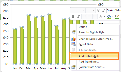
› documents › excelHow to add data labels from different column in an Excel chart? This method will guide you to manually add a data label from a cell of different column at a time in an Excel chart. 1.Right click the data series in the chart, and select Add Data Labels > Add Data Labels from the context menu to add data labels. How to Print Labels from Excel - Lifewire Select Mailings > Write & Insert Fields > Update Labels . Once you have the Excel spreadsheet and the Word document set up, you can merge the information and print your labels. Click Finish & Merge in the Finish group on the Mailings tab. Click Edit Individual Documents to preview how your printed labels will appear. Select All > OK . Custom Chart Data Labels In Excel With Formulas Follow the steps below to create the custom data labels. Select the chart label you want to change. In the formula-bar hit = (equals), select the cell reference containing your chart label's data. In this case, the first label is in cell E2. Finally, repeat for all your chart laebls. peltiertech.com › multiple-time-series-excel-chartMultiple Time Series in an Excel Chart - Peltier Tech Aug 12, 2016 · Start by selecting the monthly data set, and inserting a line chart. Excel has detected the dates and applied a Date Scale, with a spacing of 1 month and base units of 1 month (below left). Select and copy the weekly data set, select the chart, and use Paste Special to add the data to the chart (below right).

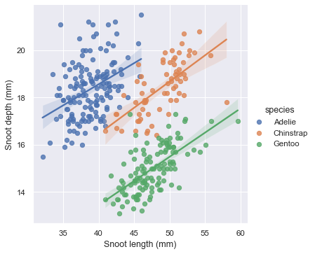
Multiple linear regression — seaborn 0.11.1 documentation

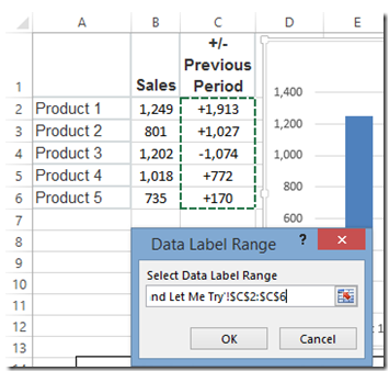
chandoo.org › wp › change-data-labels-in-chartsHow to Change Excel Chart Data Labels to Custom Values? May 05, 2010 · Now, click on any data label. This will select “all” data labels. Now click once again. At this point excel will select only one data label. Go to Formula bar, press = and point to the cell where the data label for that chart data point is defined. Repeat the process for all other data labels, one after another. See the screencast.

Data labels on Excel charts « projectwoman.com

How to Use Excel Pivot Table Label Filters To change the Pivot Table option, and allow multiple filters, follow these steps: Right-click a cell in the pivot table, and click PivotTable Options. In the PivotTable Options dialog box, click the Totals & Filters tab In the Filters section, add a check mark to 'Allow multiple filters per field.'

How to Add Data Labels in Excel - Excelchat | Excelchat

8 Types of Excel Charts and Graphs and When to Use Them Pie graphs are some of the best Excel chart types to use when you're starting out with categorized data. With that being said, however, pie charts are best used for one single data set that's broken down into categories. If you want to compare multiple data sets, it's best to stick with bar or column charts. 3. Excel Line Charts

How-to Use Data Labels from a Range in an Excel Chart - Excel Dashboard Templates

Formatting Long Labels in Excel - PolicyViz Wrapping Labels. It's easy to get your labels to wrap onto multiple lines so they fit and are readable. Let's say you have a simple data set of the population of large cities in the United States. Instead of having them stick out to the left of the chart, you'd like to wrap them on two lines, with the city above and the state below.

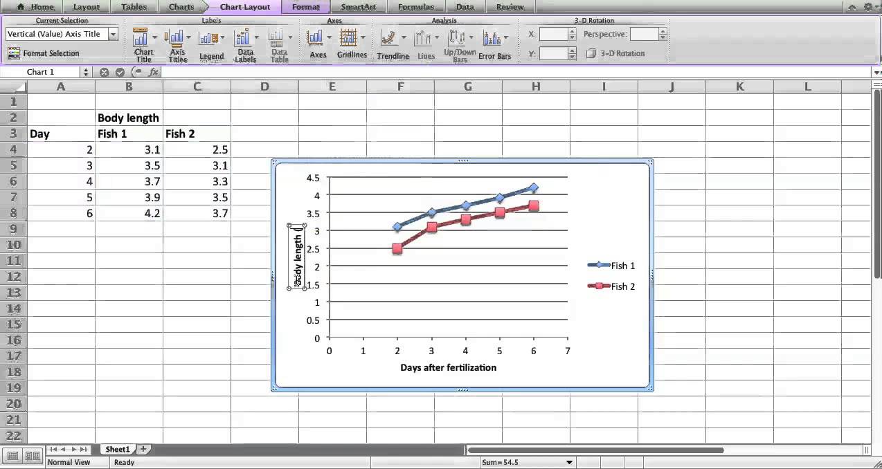
Making a scatter plot in Excel Mac 2011 - YouTube

How to Find, Highlight, and Label a Data Point in Excel Scatter Plot? By default, the data labels are the y-coordinates. Step 3: Right-click on any of the data labels. A drop-down appears. Click on the Format Data Labels… option. Step 4: Format Data Labels dialogue box appears. Under the Label Options, check the box Value from Cells . Step 5: Data Label Range dialogue-box appears.

Excel Custom Chart Labels • My Online Training Hub

How to Apply a Filter to a Chart in Microsoft Excel Select the data for your chart, not the chart itself. Go to the Home tab, click the Sort & Filter drop-down arrow in the ribbon, and choose "Filter." Click the arrow at the top of the column for the chart data you want to filter. Use the Filter section of the pop-up box to filter by color, condition, or value.

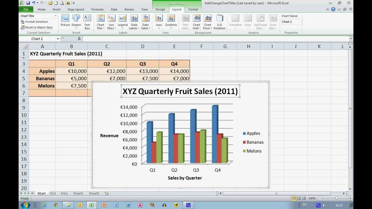
How To... Add and Change Chart Titles in Excel 2010 - YouTube

› office-addins-blog › 2015/11/05How to create a chart in Excel from multiple sheets - Ablebits Nov 05, 2015 · Supposing you have a few worksheets with revenue data for different years and you want to make a chart based on those data to visualize the general trend. 1. Create a chart based on your first sheet. Open your first Excel worksheet, select the data you want to plot in the chart, go to the Insert tab > Charts group, and choose the chart type you ...

Charts

How to Create a Bar Chart in Excel with Multiple Bars? To add data labels, go to the Chart Design ribbon, and from the Add Chart Element, options select Add Data Labels. Adding data labels will add an extra flair to your graph. You can compare the score more easily and come to a conclusion faster. You can also choose a column chart that will give you a similar result.

Chapter 3 Excel 2007/2010 Charts

Chart two columns of data on the horizontal axis Chart two columns of data on the horizontal axis. When I download my blood pressure data from my monitor I get one column for dates and another column for times within each date. I'm trying to get a chart with data points for each date and time. I don't know to create a formula for the horizontal axis which combine column A (date) and Column B ...

Enable or Disable Excel Data Labels at the click of a button - How To - PakAccountants.com

How do I add another label to an Excel chart? Add data labels Click the chart , and then click the Chart Design tab. Click Add Chart Element and select Data Labels, and then select a location for the data label option. Note: The options will differ depending on your chart type. If you want to show your data label inside a text bubble shape, click Data Callout.

How To Make A Data Table With Multiple Trials

How to Create and Customize a Treemap Chart in Microsoft Excel Either right-click the chart and pick "Format Chart Area" or double-click the chart to open the sidebar. On Windows, you'll see two handy buttons on the right of your chart when you select it. With these, you can add, remove, and reposition Chart Elements. And you can pick a style or color scheme with the Chart Styles button.

How-to Use Data Labels from a Range in an Excel Chart - Excel Dashboard Templates

Make All Of Your Excel Charts The Same Size Click the chart to select it. Chart Tools>Format- note the height and width settings of the chart. Select CTL+Click the other three charts so all four are selected. Chart>Tools Format-enter in the height and width settings noted in the first step above. The charts will now be the same size see below.

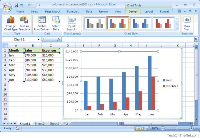
Column Chart in Excel - Easy Excel Tutorial

How to Make a Frequency Distribution Table & Graph in Excel? Prepare Your Data at First. 1: Use My FreqGen Excel Template to build a histogram automatically. 2: Frequency Distribution Table Using Pivot Table. Step 1: Inserting Pivot Table. Step 2: Place the Score field in the Rows area. Step 3: Place the Student field in the Values area.

Custom data labels in a chart | Get Digital Help - Microsoft Excel resource

5 New Charts to Visually Display Data in Excel 2019 - dummies Enter the labels and data. Put them in the order you want them to appear in the chart, from top to bottom. You can convert the range to a table to sort it more easily. Select the labels and data and then click Insert → Insert Waterfall, Funnel, Stock, Surface, or Radar Chart → Funnel. Format the chart as desired.

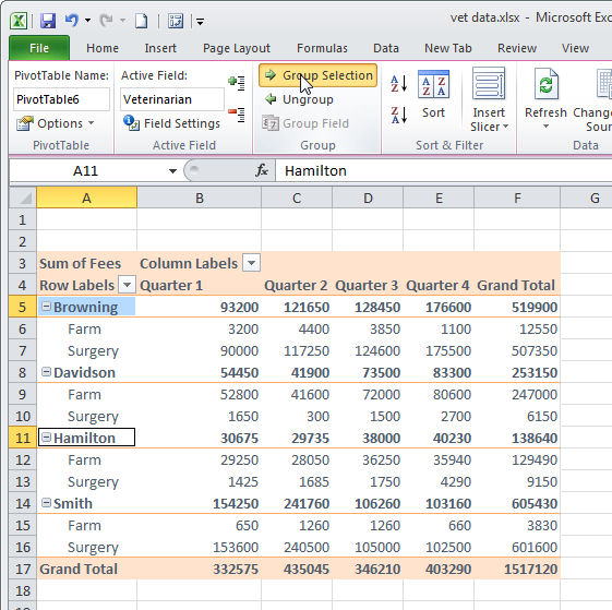
Group data in an Excel Pivot Table

Excel Waterfall Chart: How to Create One That Doesn't Suck Click inside the data table, go to " Insert " tab and click " Insert Waterfall Chart " and then click on the chart. Voila: OK, technically this is a waterfall chart, but it's not exactly what we hoped for. In the legend we see Excel 2016 has 3 types of columns in a waterfall chart: Increase. Decrease.

Do any kind of work on ms excel by Sagarkumar904

DataLabel object (Excel) | Microsoft Docs With Charts ("chart1") With .SeriesCollection (1).Points (2) .HasDataLabel = True .DataLabel.Text = "Saturday" End With End With On a trendline, the DataLabel property returns the text shown with the trendline. This can be the equation, the R-squared value, or both (if both are showing).

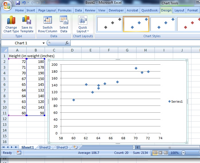
Scatter Plot / Scatter Chart: Definition, Examples, Excel/TI-83/TI-89/SPSS - Statistics How To

How to set multiple series labels at once - Microsoft Tech Community Click anywhere in the chart. On the Chart Design tab of the ribbon, in the Data group, click Select Data. Click in the 'Chart data range' box. Select the range containing both the series names and the series values. Click OK. If this doesn't work, press Ctrl+Z to undo the change. 0 Likes Reply Nathan1123130 replied to Hans Vogelaar

How to Make Excel Charts More Intuitive by Adding Data Labels and Tables - Data Recovery Blog

How to Create a Dynamic Chart Title in Excel Select chart title in your chart. Go to the formula bar and type =. Select the cell which you want to link with chart title. Hit enter. Related: Combine Cell Link and Text to Create a Dynamic Chart Title Now, let me show you how to combine a cell and a text to create a dynamic chart title.

Share :